SM + Scalar | Exotic Higgs Decays

The Model

A particularly simple extension of the SM is to add to it one real scalar singlet S. This model can easily produce non-trivial exotic Higgs decays, since 1.) the Higgs can decay to pair of singlets; and 2.) the singlet decays to SM particles A simple model that could be conceived involves an additional real singlet added to the SM. At the renormalizable level, gauge invariance allows the singlet S to couple only to itself and to H^† H ≡ |H|². The resulting potential is given by

where V(S) is a general quartic polynomial that may give S a vacuum expectation value. The couplings k and ζ generate mixings between H and S. Assuming those mixings are small, we identify the uneaten doublet degree of freedom to be the SM-like Higgs with m_h = 125 GeV and take the singlet field to have a mass below m_h/2. The small mixings give mass eigenstates h and s, which are mostly doublet- and singlet-like, respectively. The decays h → s s are generated by an effective cubic term, and s decays to SM particles via its doublet admixture.

Several variations of the model presented above are possible, for example, additional symmetries could be imposed to forbid certain terms in the potential leading to an even simpler version of this model, or one could take the singlet to be a complex field although the phenomenology remains unchanged.

Phenomenology

After electroweak symmetry breaking there are two relevant mass-eigenstates: the SM-like scalar h at 125 GeV containing a small admixture of S, and the mostly-singlet scalar s containing a small admixture of H. The phenomenology of any SM+S model can be, generally speaking, captured in terms of three parameters:

The effective Lagrangian contains a term of the form μ_v h s s, which gives h → s s with BR(h→ exotic) determined by μ_v.
The singlet's mass m_s affects BR(h→ exotic) and the type of SM final states available for s → SM.
The mixing angle between S and H, denoted here by θ_S, determines the overall width of s→SM. If s cannot decay to other non-SM fields, θ_S controls its lifetime.

Screen Shot 2013-12-12 at 2.46.04 PM

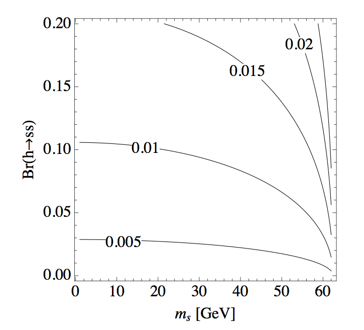
Figure 1: Size of the cubic coupling μ_v in units of Higgs expectation value v to yield the indicated h → s s branching fraction as a function of singlet mass.

The partial width of Higgs decay to singlets (see arXiv:1312.4992 for details) is plotted as a function of the singlet mass for different values of μ_v/v in Fig. 1, where v is the Higgs vacuum expectation value. The individual decay widths of s to SM particles are readily computed using existing calculations for Higgs decays, e.g. [2,3] and mostly dominated by decay to heavy fermions for m_s < m_h/2 when kinematically allowed. BR(s→ SM) and BR(h→ ss → SM) are shown for m_s > 1 GeV in Fig. 2 on the left and right, respectively. The theoretical calculations become increasingly inaccurate as m_s is lowered to ∼ 1 GeV, where perturbative QCD breaks down, or when m_s is close to a hadronic resonance, which can enhance the decay rates [4].

Let us briefly comment on the region m_s < 1 GeV which is not shown in Fig. 2. For m_s above the pion threshold, the singlet can decay to some combination of hadrons, which are boosted due to the large mass difference between the singlet and h. The resulting two-track jet may look like a low-quality hadronic τ-decay. Between the muon and pion thresholds (210 MeV <~m_s <~270 MeV), the dominant decay is to μ⁺μ⁻, while for m_s <~210 MeV, the dominant decay is to e⁺e⁻. Photons are the only possible final state for m_s < 2 m_e , in which case the scalar is detector-stable.

Screen Shot 2013-12-12 at 2.55.54 PM

Figure 2 (left)

Figure 2 (right)

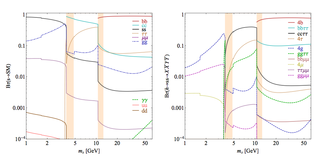
Figure 2: Left: Branching ratios of a CP-even scalar singlet to SM particles, as function of m_s. Right: Branching ratios of exotic decays of the 125 GeV Higgs boson as function of m_s, in the SM + Scalar model described in the text, scaled to BR(h→ ss) = 1. Hadronization effects likely invalidate our simple calculation in the shaded regions.

It should be pointed out that the partial decay widths are affected by the parity of s, however, the BR of s decaying to SM particles remains unchanged. Further, the decay width of s is suppressed by a factor of sin² θ_s which opens the possibility of displaced vertices for θ <~10⁻⁶.

Further details of the branching ratio calculation can be found in Section 1.3.2 and Appendix A of arXiv:1312.4992, which also includes a more detailed discussion of pseudoscalar decays.

MadGraph Model

We have constructed a validated MadGraph 5 model for the SM + vector + dark higgs scenario outlined here. Taking kinetic mixing to zero reduces this model to the SM+S scenario of this section. This can be used for signal generation in experimental and phenomenological studies.

Link to MadGraph5 model for SM + S + V

References

: [1]LHC New Physics Working Group, D. Alves et. al., Simplified Models for LHC New Physics Searches, J.Phys. G39 (2012) 105005, [arXiv:1105.2838].
: [2]A. Djouadi, The Anatomy of Electro-Weak Symmetry Breaking. II: The Higgs bosons in the Minimal Supersymmetric Model, [hep-ph/0503173v2].
: [3]A. Djouadi, The Anatomy of Electro-Weak Symmetry Breaking. I: The Higgs boson in the Standard Model, [hep-ph/0503172v2].
: [4]J. Gunion, H. Haber, G. Kane, and S. Dawson, The Higgs Hunter's Guide. Frontiers in Physics, V. 80. Perseus Pub., 2000.

File translated from T_EX by T_TH, version 4.03. On 12 Dec 2013, 14:20.